| 일 | 월 | 화 | 수 | 목 | 금 | 토 |
|---|---|---|---|---|---|---|
| 1 | 2 | 3 | ||||
| 4 | 5 | 6 | 7 | 8 | 9 | 10 |
| 11 | 12 | 13 | 14 | 15 | 16 | 17 |
| 18 | 19 | 20 | 21 | 22 | 23 | 24 |
| 25 | 26 | 27 | 28 | 29 | 30 | 31 |
- drug muggers
- ChIPseq
- 비타민 C
- single cell rnaseq
- js
- scRNAseq
- github
- DataFrame
- ngs
- scRNAseq analysis
- EdgeR
- javascript
- cellranger
- julia
- 싱글셀 분석
- PYTHON
- drug development
- python matplotlib
- single cell
- HTML
- CUT&RUN
- CSS
- single cell analysis
- matplotlib
- Batch effect
- Bioinformatics
- Git
- CUTandRUN
- pandas
- MACS2
- Today
- Total
바이오 대표
[scRNAseq 논문] 싱글셀 데이터 분석 bioinformatician 관점 “Current best practices in single-cell RNA-seq analysis: a tutorial” 2019 본문
[scRNAseq 논문] 싱글셀 데이터 분석 bioinformatician 관점 “Current best practices in single-cell RNA-seq analysis: a tutorial” 2019
바이오 대표 2023. 2. 23. 12:12
해당 글은 "Current best practices in single-cell RNA-seqanalysis: a tutorial" https://www.embopress.org/doi/epdf/10.15252/msb.20188746" 를 요약 정리한 글입니다.
전체 흐름
scRNAseq analysis tools increase → lack of standardization (+ dependency of language)
The paper introduces the typical scRNAseq analysis steps as current best-practice recommendations. 처음 분석을 하시는 분들께 어느정도 가이드라인이 되는 페이퍼라고 생각한다.
- count matrix
- pre-processing
- QC, normalization, data correction, feature selection, dimensionality reduction
- cell - and gene-level downstream analysis
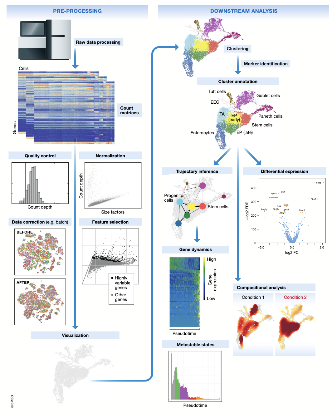
Pre-processing and visualization
Raw data ——————————————→ count matrix
- wet lab (tissue to count)
Raw data processing pipelines:
- Cell Ranger (or others)
- read QC, assigning reads to the cellular barcodes, mRNA molecules of origin (demultiplexing), genome alignment, quantification
- Demultiplexing def.
- Demultiplexing in sequencing: sorting reads into different FASTQ files for different libraries pooled into a single sequencing runs
- Separating out multiple samples pooled into a single library
- Tools https://www.10xgenomics.com/resources/analysis-guides/bioinformatics-tools-for-sample-demultiplexing
Result Count Matrix:
#of barcodes(cells) x #of transcripts
Quality Control
= doublets, low-quality cells (dying cells) 제거를 위함이고 보통, scrublet, doubletFinder and doubletDecon 이 사용된다.
QC covariates (main):
- the #of counts per barcode (count depth)
- the #of genes per barcode - count가 하나 이상인 gene 개수
- the fraction of counts from mt genes per barcode
고려사항:
- 해당 covariates를 각각 생각하면 안되고 consider jointly (biological 의미가 있을 수 있다).
- Start w/ permissive QC
- distrbution QC 가 샘플마다 다르면, 각 샘플마다 다른 threshold 취하기
** For Heterogeneous cell population may exhibit multiple QC covariate peaks
Normalization
[1] GOAL: normalization between cells (count depth)
방법 : global scaling, linear normalization
Assumption: each cell has an equal number of mRNA molecules/count depth
- High-counted filtering CPM (Wein- reb et al , 2018)
- count’s 5% 이상을 차지하는 genes 들은 size factor 계산할때 포함 안함
- allow counts variability in a few highly expressed genes
- Scran (Lun et al, 2016a) 현존 탑!!
- limits variability to fewer than 50% of genes being differentially expressed between cells,
- :) in a small-scale comparision
- batch correction 뛰어남
** strong batch effect 를 보이는 데이터에는 Non-linear normalization methods 효과 좋음 (Cole et al, 2019)
Full-length data - TPM normalization
3’end - scran 사용 추천
[2] gene normalization: scaling gene counts to z scores (0 mean, unit variance)
Assumption: all genes are weighted equally
**Seurat 에서는 사용, 다른데서는 반대
⇒ normalization 후에는 보통 log(x+1) transform 을 해준다
- distance = log fold change
- mitigates mean-variance relationship
- reduce the skewness of the data
주의! test group 간의 size factor distribution이 크게 차이가 나면 거짓부렁 결과보여줄수 있음
Feature selection, dimensionality reduction, and visualization
Human scRNAseq can contain up to 25,000 genes — QC —> ~ 15,000
GOAL: 엄청난 sparse/dimension 데이터를 유의미하게 함축
Feature Selection
- highly variable genes (HVGs) 를 이용하여 downstream analysis 하는 것인데 high # of HVGs 추전
- HOW?
- binned by gene’s mean expression → for each bin, genes with the highest variance-to-mean ratio are selected
- from count data (Seurat) //question what is Seurat default gene number?
- from log-transformed data (Cell Ranger)
- ** 데이터가 z-score normalization 이 되있으면 적용 불가
- HOW?
Dimensionality reduction
- Summarization
- PCA (principle component analysis)
- linear approach, reduce dimension by maximizing the captured residual variance in each further dimension
- As pre-step for non-linear dimensionality
- distance 유의미
- Diffusion maps
- non-linear approach, alternative to PCA for trajectory inference summarization
- Continuous process 데이터에 굿 (differentiation is of interest)
- PCA (principle component analysis)
- Visualization (non-linear)
- t-SNE: local similarity 에 초점
- UMAP: 현존 짱!! *2D 이상으로도 데이터 summarize 된다 (발전 가능성!)
- SRPING: graph-based tools
- PAGA: for coarse-grained visualization (for large numbers of cells)
Downstream analysis
Cluster analysis - explain the heterogeneity
Trajectory analysis - explain the dynamic process
[1] cell level analysis
Clustering: Louvain algorithm + sc KNN graphs (Seurat, Scanpy default method) or flow/mass cytometry
Cluster annotation
Marker genes → cell identities (원하는 cluster resolution을 염두해 두고 진행)
- DB 이용
- mouse brain atlas (Zeisel et al, 2018) and human cell atlas (Regev et al, 2017)
- DE testing 을 이용해서 marker gene 찾기
- Wilcoxon rank-sum test/t-test → top up-regulated genes (rank) for each cluster
- annotated by comparing marker genes via enrichment tests, Jaccard index
- ** permutation test (assumption: all samples come from the same distribution)
- Automated cluster annotation (depends on condition)
- HOW?
- Comparing gene expression profiles of annotated reference clusters (reference 있으면 추천)
- scmap (Kiselev et al, 2018b) or Garnett (preprint: Pliner et al, 2019
- HOW?
**p-value inflated 될수도있으니 이것만 가지고 Marker gene 구하면 안댐
Compositional analysis
cluster 의 cell proportion 을 중심으로 분석
Trajectory Analysis
For dynamic models of gene expression - cellular diversity (cell transition, differentiation, ,,)
- HOW?
- Monocle. (BEAM), Wanderlust, PAGA (visualization)
- https://www.nature.com/articles/s41587-019-0071-9
[2] gene-level analysis
- DEG
- HOW? weighted bulk DE analysis
- EdgeR, DESeq2 + ZINB-wave weights or (limma-voom / MAST)
- Gene Set Analysis
- DEGs 가 너무 많을때, characteristic에 따라 grouping → testing
- DB: MsigDV, GO, GO consortium, KEGG, Reactome
- for single cell - to perform ligand-receptor analysis use of paired gene labels
- DB: CellPhonDB
- Gene Regulatory Network (아직 부족하다)
- based on co-expression (correlation,
- HOW?
- SCONE, SCENIC, PIDC

